library(metaverse)
#> -- Attaching packages ------------------------------------------------------------------------------------------- metaverse 0.0.1 --
#> v robvis       0.1.0          v metadat      0.1.0     
#> v metafor      2.0.0          v broom        0.5.2.9001
#> v tidymeta     0.1.0.9000     v pubBias      0.0.1     
#> v litsearchr   0.1.0          v metaDigitise 1.0.0     
#> v revtools     0.3.0

Model objects can be challenging to work with in their raw form in R. The broom:: package provides tools to extract commonly desired model output in table form:

tidy() summarizes information about model components

glance() reports information about the entire model

augment() adds information about observations to a dataset ()

demonstration

We begin by creating a random-effects model object via metafor::, which is included in the metaverse::.

# grab a dataset from metafor
# from the metafor homepage
dat.bcg <- metafor::dat.bcg
ma_model <-
  escalc(
    measure = "RR",
    ai = tpos,
    bi = tneg,
    ci = cpos,
    di = cneg,
    data = dat.bcg
  ) %>% rma(yi, vi, data = ., method = "EB")

broom functionality

We can now use broom:: functionality to manage the output in a common format

tidy() summarizes information about model components

ma_model %>% tidy() %>% knitr::kable()

study	type	estimate	std.error	statistic	p.value	conf.low	conf.high
1	study	-0.8893113	0.5706004	-1.5585538	NA	-2.0076675	0.2290448
2	study	-1.5853887	0.4411135	-3.5940606	NA	-2.4499552	-0.7208221
3	study	-1.3480731	0.6444905	-2.0916883	NA	-2.6112513	-0.0848950
4	study	-1.4415512	0.1414568	-10.1907507	NA	-1.7188015	-1.1643009
5	study	-0.2175473	0.2262966	-0.9613369	NA	-0.6610806	0.2259860
6	study	-0.7861156	0.0831001	-9.4598689	NA	-0.9489887	-0.6232425
7	study	-1.6208982	0.4722470	-3.4323101	NA	-2.5464854	-0.6953111
8	study	0.0119523	0.0629411	0.1898972	NA	-0.1114099	0.1353146
9	study	-0.4694176	0.2375589	-1.9760057	NA	-0.9350245	-0.0038108
10	study	-1.3713448	0.2702310	-5.0747131	NA	-1.9009878	-0.8417018
11	study	-0.3393588	0.1114101	-3.0460324	NA	-0.5577186	-0.1209990
12	study	0.4459134	0.7297300	0.6110663	NA	-0.9843311	1.8761579
13	study	-0.0173139	0.2672165	-0.0647937	NA	-0.5410487	0.5064208
Overall	summary	-0.7149682	0.1808922	-3.9524542	7.74e-05	-1.0695104	-0.3604260

glance() reports information about the entire model

ma_model %>% glance()  %>% knitr::kable()

	i.squared	h.squared	tau.squared	logLik	deviance	AIC	BIC	AICc
ML	92.33034	13.03839	0.3180685	-12.69434	37.17454	29.38867	30.51857	30.58867

augment() adds information about observations to a dataset ()

ma_model %>% augment() %>% knitr::kable()

y	.fitted	.se.fit	conf.low.fit	conf.high.fit	.resid	.hat	.cooksd	.std.resid	.dffits	.cov.ratio	tau.squared.del	qe.del	.weight	.dfbetas
-0.8893113	-0.8011218	0.4114171	-1.6074845	0.0052409	-0.1743432	0.0508379	0.0012736	-0.2131968	-0.0346868	1.1559082	0.3557591	151.58257	5.083791	-0.0341029
-1.5853887	-1.2550121	0.3541752	-1.9491828	-0.5608415	-0.8704205	0.0638291	0.1127214	-1.2873585	-0.3433276	1.0063461	0.2956598	145.31761	6.382915	-0.3457374
-1.3480731	-0.9895260	0.4366086	-1.8452632	-0.1337889	-0.6331050	0.0446146	0.0251089	-0.7465310	-0.1566895	1.0917526	0.3347164	150.19704	4.461462	-0.1552226
-1.4415512	-1.3985465	0.1376238	-1.6682843	-1.1288088	-0.7265830	0.0967881	0.2072828	-1.3855766	-0.4774554	1.0222047	0.2873981	96.56260	9.678813	-0.4741775
-0.2175473	-0.2865278	0.2115132	-0.7010859	0.1280304	0.4974208	0.0886106	0.0741674	0.8469886	0.2685559	1.1261213	0.3285400	151.32001	8.861056	0.2687968
-0.7861156	-0.7846037	0.0823022	-0.9459131	-0.6232944	-0.0711474	0.1006911	0.0005643	-0.1187102	-0.0224454	1.2188854	0.3571164	128.18666	10.069106	-0.0226653
-1.6208982	-1.2475045	0.3696700	-1.9720444	-0.5229646	-0.9059301	0.0604747	0.1086793	-1.3017502	-0.3371001	0.9993512	0.2944645	145.82964	6.047468	-0.3400323
0.0119523	0.0030098	0.0625923	-0.1196688	0.1256885	0.7269205	0.1016116	0.1977841	1.4241116	0.4702238	1.0191957	0.2840955	67.98581	10.161159	0.4653240
-0.4694176	-0.5064199	0.2206199	-0.9388269	-0.0740129	0.2455505	0.0873745	0.0211744	0.4071677	0.1395737	1.1853279	0.3506259	152.20506	8.737450	0.1398780
-1.3713448	-1.2487864	0.2460294	-1.7309951	-0.7665777	-0.6563766	0.0836680	0.1127990	-1.1093255	-0.3394145	1.0687229	0.3099100	139.82707	8.366799	-0.3393882
-0.3393588	-0.3534660	0.1095089	-0.5680994	-0.1388325	0.3756093	0.0990133	0.0559519	0.6703185	0.2293929	1.1673499	0.3389876	151.46550	9.901331	0.2305232
0.4459134	-0.2808616	0.4603840	-1.1831976	0.6214744	1.1608816	0.0384705	0.0553645	1.2982901	0.2385894	0.9770428	0.2947524	150.78683	3.847046	0.2426011
-0.0173139	-0.1452194	0.2437487	-0.6229582	0.3325193	0.6976542	0.0840160	0.1196453	1.1878730	0.3524348	1.0520605	0.3037544	149.78842	8.401603	0.3523639

Analysis

We can use functions from tidymeta:: to conduct subgroup meta-analyses

ma_model_wkh <- metafor::dat.bcg


ma <- ma_model_wkh %>% 
  escalc(
    measure = "RR",
    ai = tpos,
    bi = tneg,
    ci = cpos,
    di = cneg,
    data = .) %>%
  dplyr::group_by(alloc) %>% 
  meta_analysis(yi = yi, vi = vi, slab = author, exponentiate = TRUE) 

ma
#> # A tibble: 17 x 11
#>    alloc study type  estimate std.error statistic  p.value conf.low
#>    <chr> <chr> <chr>    <dbl>     <dbl>     <dbl>    <dbl>    <dbl>
#>  1 rand~ Aron~ study    0.411    0.571    -1.56   NA         0.134 
#>  2 rand~ Ferg~ study    0.205    0.441    -3.59   NA         0.0863
#>  3 rand~ Rose~ study    0.260    0.644    -2.09   NA         0.0734
#>  4 rand~ Hart~ study    0.237    0.141   -10.2    NA         0.179 
#>  5 rand~ Vand~ study    0.198    0.472    -3.43   NA         0.0784
#>  6 rand~ TPT ~ study    1.01     0.0629    0.190  NA         0.895 
#>  7 rand~ Coet~ study    0.625    0.238    -1.98   NA         0.393 
#>  8 rand~ Subg~ summ~    0.379    0.276    -3.52    4.34e-4   0.221 
#>  9 alte~ Frim~ study    0.804    0.226    -0.961  NA         0.516 
#> 10 alte~ Stei~ study    0.456    0.0831   -9.46   NA         0.387 
#> 11 alte~ Subg~ summ~    0.582    0.282    -1.92    5.48e-2   0.335 
#> 12 syst~ Rose~ study    0.254    0.270    -5.07   NA         0.149 
#> 13 syst~ Coms~ study    0.712    0.111    -3.05   NA         0.573 
#> 14 syst~ Coms~ study    1.56     0.730     0.611  NA         0.374 
#> 15 syst~ Coms~ study    0.983    0.267    -0.0648 NA         0.582 
#> 16 syst~ Subg~ summ~    0.654    0.360    -1.18    2.38e-1   0.323 
#> 17 Summ~ Over~ summ~    0.489    0.180    -3.97    7.05e-5   0.344 
#> # ... with 3 more variables: conf.high <dbl>, meta <list>, weight <dbl>

Forest Plot

tidymeta:: also has some handy ggplot based graphics for meta-analysis. Graph elements can be added using ggplot2 geoms.

fp <- ma %>% 
  forest_plot(group = alloc) +
  ggplot2::geom_vline(xintercept = 0, linetype = "dashed") +
  ggplot2::xlab("Effect sizes") +
  ggplot2::labs(title = "Forest plot of effect size by allocation type")

fp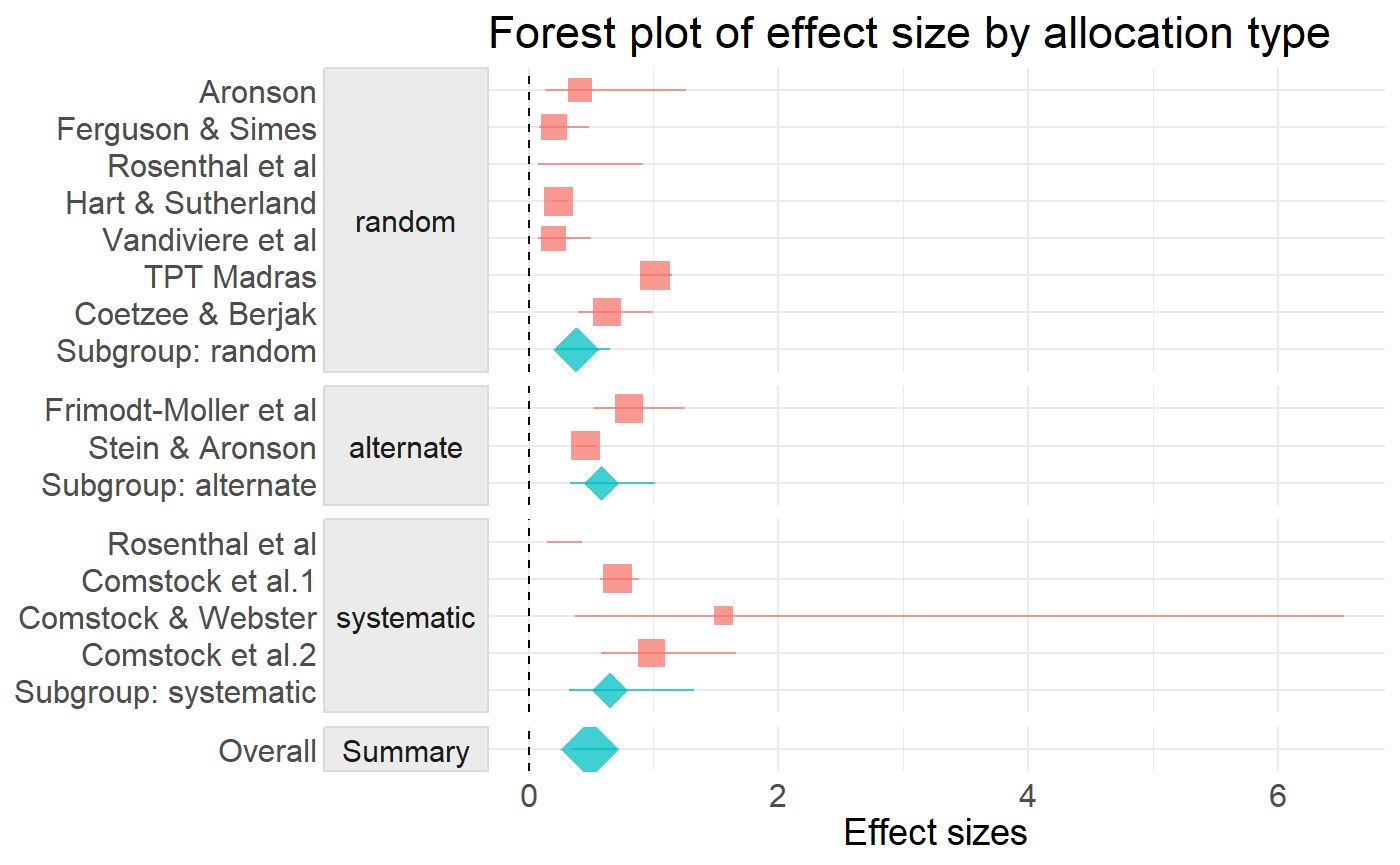

Publication Bias

Estimates the Vevea and Hedges (1995) weight-function model using the pubBias:: package.

weightrMeta(ma)
#> 
#> Unadjusted Model (k = 17):
#> 
#> tau^2 (estimated amount of total heterogeneity): 0.0000 (SE = 0.0516)
#> tau (square root of estimated tau^2 value):  0.0000
#> 
#> Model Results:
#> 
#>           estimate std.error z-stat      p-val  ci.lb  ci.ub
#> Intercept   0.6212    0.1138  5.458 4.8221e-08 0.3981 0.8442
#> 
#> Adjusted Model (k = 17):
#> 
#> tau^2 (estimated amount of total heterogeneity): 0.0000 (SE =   NaN)
#> tau (square root of estimated tau^2 value):  0.0000
#> 
#> Model Results:
#> 
#>               estimate std.error z-stat     p-val   ci.lb  ci.ub
#> Intercept       0.8846    0.1295  6.833 8.314e-12  0.6309  1.138
#> 0.025 < p < 1  10.6636   10.4276  1.023   0.30648 -9.7741 31.101
#> 
#> Likelihood Ratio Test:
#> X^2(df = 1) = 5.590652, p-val = 0.018057

Meta-Analysis Workflow

Charles T. Gray, Malcolm Barrett, W. Kyle Hamilton

2019-04-18

demonstration

broom functionality

Analysis

Forest Plot

Publication Bias

Contents